Evaluation of Binary Classifiers
Chen Hao posted on 15 Mar 20161. Contingency Table
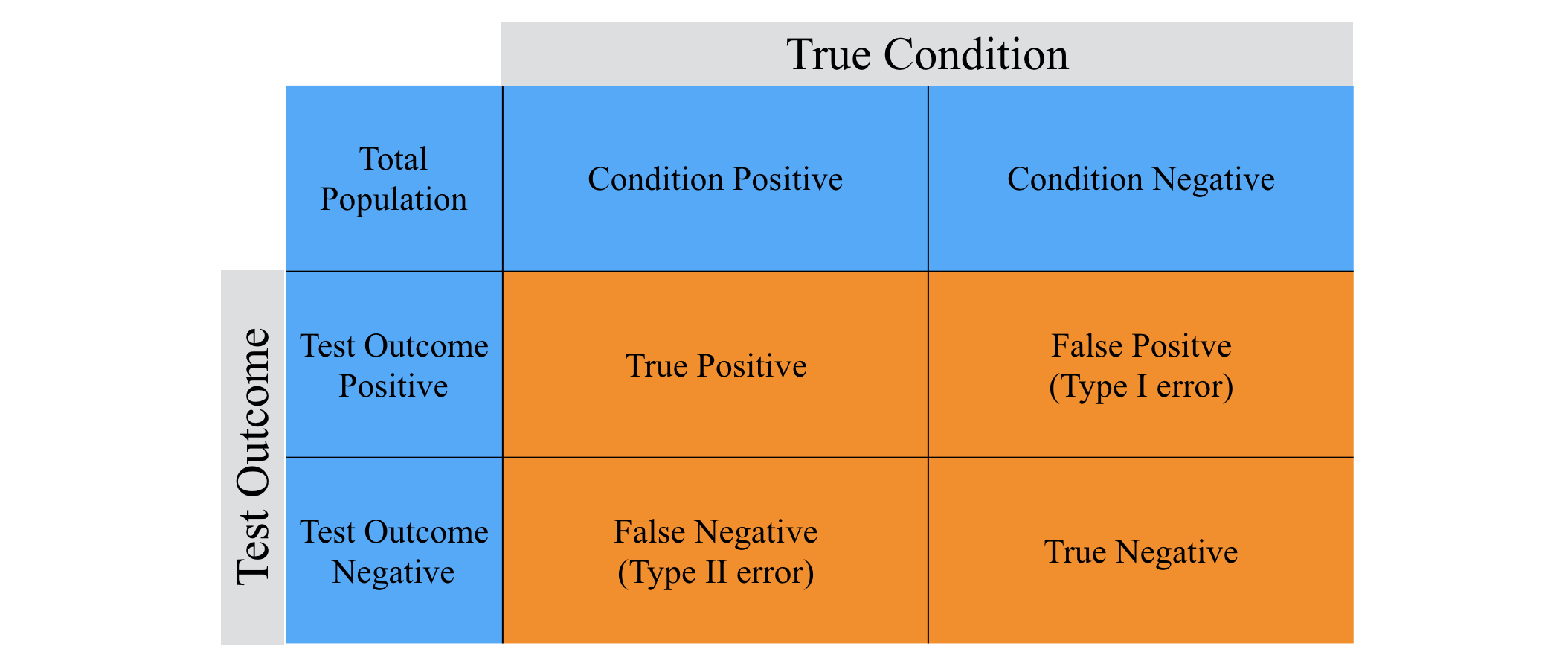
The outcomes of binary classification can be formulated in a 2×2 contingency table or confusion matrix, as follows:
There are many metrics that can be used to measure the performance of a classifier; different fields have different preferences for specific metrics due to different goals. For example, in medicine sensitivity and specificity are often used, while in information retrieval precision and recall are preferred.
Precision and specificity are two different metrics:
\[Precision = PPV = \frac{\sum True Positive}{\sum Test Outcome Positve}\] \[Specificity = TNR = \frac{\sum True Negative}{\sum Condition Negative}\]But recall and sensitivity refers to the same metric - the true positive rate:
\[Recall = Sensitivity = TPR = \frac{\sum True Positve}{\sum Condition Positve}\]2. F-measure
A measure that combines precision and recall is the F-measure. The general form of F-measure(or F_beta measure, for non-negative real values of beta) is:
\[F_{\beta} = (1 + \beta^2) \frac{Precision \cdot Recall}{\beta^2 \cdot Precision + Recall}\]The most commonly used form of F-measure is F_1 measure, where recall and precision are evenly weighted. Two other commonly used F measures are the F_2 measure, which weights recall higher than precision, and the F_0.5 measure, which puts more emphasis on precision than recall.
3. Accuracy
Accuracy measures how well a binary classification test correctly identifies or excludes a condition. That is, the accuracy is the proportion of true results (both true positives and true negatives) among the total number of cases examined.
\[Accuracy(ACC) = \frac{\sum True Positive + \sum True Negative}{\sum Total Population}\]Another useful performance measure is the balanced accuracy which avoids inflated performance estimates on imbalanced datasets. It is defined as the arithmetic mean of sensitivity and specificity, or the average accuracy obtained on either class:
\[Balanced Accuracy = \frac{Sensitivity + Specificity}{2}\]If the classifier performs equally well on either class, this term reduces to the conventional accuracy (i.e., the number of correct predictions divided by the total number of predictions). In contrast, if the conventional accuracy is above chance only because the classifier takes advantage of an imbalanced test set, then the balanced accuracy, as appropriate, will drop to chance. A closely related chance corrected measure is informedness:
\[Informedness = Sensitivity + Specificity - 1 = 2 \times Balanced Accuracy - 1\]4. kappa
A direct approach to debiasing and renormalizing Accuracy is Cohen’s kappa, whilst Informedness has been shown to be a Kappa-family debiased renormalization of Recall. Informedness and Kappa have the advantage that chance level is defined to be 0, and they have the form of a probability. Informedness has the stronger property that it is the probability that an informed decision is made (rather than a guess), when positive. When negative this is still true for the absolutely value of Informedness, but the information has been used to force an incorrect response.
The formula for Kappa is:
\[Kappa = \frac{Total Accuracy - Random Accuracy}{1 - Random Accuracy}\]where:
\[Total Accuracy = \frac{\sum True Positive + \sum True Negative}{\sum Total Population} \\ Random Accuracy = \frac{(TN + FP)\times(TN + FN) + (FN + TP)\times(FP + TP)}{\sum Total Population \times \sum Total Population}\]Code Example
require(caret)
## build a starting dataframe
df <- data.frame(act = rep(LETTERS[1:2], each=10),
                 pred = rep(sample(LETTERS[1:2], 20, replace=T)))

## create working frequency table
tab <- table(df)

## A balanced dataset
tab[1,1] <- 45
tab[1,2] <- 5
tab[2,1] <- 5
tab[2,2] <- 45

caret::confusionMatrix(tab)
# Confusion Matrix and Statistics
#
# pred
# act  A  B
# A 45  5
# B  5 45
#
# Accuracy : 0.9
# Kappa : 0.8

## An unbalanced datasest
tab[1,1] <- 85
tab[1,2] <- 5
tab[2,1] <- 5
tab[2,2] <- 5

caret::confusionMatrix(tab)
# Confusion Matrix and Statistics
#
# pred
# act  A  B
# A 85  5
# B  5  5
#
# Accuracy : 0.9
# Kappa : 0.444
As you can see, you can have the exact same accuracy with two different datasets but very different Kappa. The idea herein being, with unbalanced data, there is a higher chance you will randomly classify the less common group so this should be accounted for in your evaluation of the model.
5. ROC
For 2–class models, Receiver Operating Characteristic (ROC) curves can be used to characterize model performance. It’s a curve plot which shows the true positive rate (TPR) (or $Sensitivity$) against the false positive rate (FPR) (or $1 - Specificity$) at various threshold settings. When using normalized units, the area under the curve (often referred to as AUC) is used as a metric to evaluate the classifier. The more closer to 1 of AUC, the better the classifier performs.