Visual Comparation of Different Transformation Methods for Cytometry Data

Chen Hao posted on 25 Jul 2016

Introduction

In biotechnology, flow cytometry is a laser- or impedance-based, biophysical technology employed in cell counting, cell sorting, biomarker detection and protein engineering, by suspending cells in a stream of fluid and passing them by an electronic detection apparatus. It allows simultaneous multiparametric analysis of the physical and chemical characteristics of up to thousands of particles per second. [1]

Flow cytometry measurements can vary over several orders of magnitude, cell populations can have variances that depend on their mean fluorescence intensities, and may exhibit heavily-skewed distributions. Consequently, the choice of data transformation can influence the output of subsequent analysis. An appropriate data transformation aids in data visualization and gating of cell populations across the range of data. [2]

BioConductor flowCore which is the most bacis R pacakge for parsing FCM data. It provides many different transfromations including linearTransform, lnTransform, logTransform, quadraticTransform, arcsinhTransform, biexponentialTransform, logicleTransform.

As stated in [3], The goal of visualizing data of a measured parameter is to determine the actual probability function (APF) of the property being investigated. However the APF is never known, the selection of a proper transformation and parameters tuning is mainly determined by visual checking of the distribution to see if the populations are clearly segerated.

For this post, the seven transformation methods provided in flowCore are explored, parameters for each transformation are slightly investigated to gain a rough understanding of their theories and the corresponding effects. At the end, a shiny APP is provided to visually and interactively compare the two most popular transformations (logicle and arcsin) for a given FCS dataset.

Loading the raw data of a FCS file

library(flowCore)
library(ggplot2)
file <- "~/Ranalysis/Sanofi Day 0 Myeloid panel_SNF002 D0.fcs"
fcs <- read.FCS(file, transformation = FALSE)

## Error in read.FCS(file, transformation = FALSE): '~/Ranalysis/Sanofi Day 0 Myeloid panel_SNF002 D0.fcs' is not a valid file

Summary Information of the FCS data

fs <- pData(fcs@parameters)

## Error in pData(fcs@parameters): object 'fcs' not found

fs$minExprs <- apply(fcs@exprs, 2, min)

## Error in apply(fcs@exprs, 2, min): object 'fcs' not found

fs$maxExprs <- apply(fcs@exprs, 2, max)

## Error in apply(fcs@exprs, 2, max): object 'fcs' not found

fs$range <- NULL

## Error in fs$range <- NULL: object 'fs' not found

fs

## Error in eval(expr, envir, enclos): object 'fs' not found

Linear Transformation

The formula for linear transformation is x <- a*x+b, and the crrosponding funciton is linearTransform(transformationId="defaultLinearTransform", a = 1, b = 0).

Transformation function

ggplot(data.frame(x=c(-5,5)), aes(x)) +
  stat_function(fun=function(x) 1*x+0, geom="line", aes(colour="a=1,b=0")) +
  stat_function(fun=function(x) 2*x+0, geom="line", aes(colour="a=2,b=0")) +
  stat_function(fun=function(x) 2*x+5, geom="line", aes(colour="a=2,b=5")) +
  scale_colour_manual(name="a*x+b", values=c("a=1,b=0"="blue","a=2,b=0"="red", "a=2,b=5"="green")) +
    theme_bw() + geom_hline(yintercept = 0, colour = "gray20") + geom_vline(xintercept = 0, colour = "gray20") + coord_fixed()

plot of chunk unnamed-chunk-3

Example

linearTrans <- linearTransform(transformationId="Linear-transformation", a=0.00001, b=1)
lt_fcs <- transform(fcs, transformList('FSC-H' ,linearTrans))

## Error in transform(fcs, transformList("FSC-H", linearTrans)): object 'fcs' not found

par(mfrow=c(1,2))
plot(density(fcs@exprs[ ,'FSC-H']), main = "Before Transformation")

## Error in density(fcs@exprs[, "FSC-H"]): object 'fcs' not found

plot(density(lt_fcs@exprs[ ,'FSC-H']), main = "After Transformation")

## Error in density(lt_fcs@exprs[, "FSC-H"]): object 'lt_fcs' not found

Natural Logarithm Transformation (ln transformation)

The formula for ln transformation if x<-log(x)*(r/d), and the crrosponding function is lnTransform(transformationId="defaultLnTransform", r=1, d=1).

Transformation function

ggplot(data.frame(x=c(1e-20,10)), aes(x)) +
  stat_function(fun=function(x) log(x)*(1/1), geom="line", aes(colour="r=1,d=1")) +
  stat_function(fun=function(x) log(x)*(2/1), geom="line", aes(colour="r=2,d=1")) +
  stat_function(fun=function(x) log(x)*(1/2), geom="line", aes(colour="r=1,d=2")) +
  scale_colour_manual(name="log(x)*(r/d)", values=c("r=1,d=1"="blue","r=2,d=1"="red", "r=1,d=2"="green")) + 
    theme_bw() + geom_hline(yintercept = 0, colour = "gray20") + geom_vline(xintercept = 0, colour = "gray20")

plot of chunk unnamed-chunk-5

Example

lnTrans <- lnTransform(transformationId="ln-transformation", r=1, d=1)
ln_fcs <- transform(fcs, transformList('FSC-H', lnTrans))

## Error in transform(fcs, transformList("FSC-H", lnTrans)): object 'fcs' not found

par(mfrow=c(1,2))
plot(density(fcs@exprs[ ,'FSC-H']), main = "Before Transformation")

## Error in density(fcs@exprs[, "FSC-H"]): object 'fcs' not found

plot(density(ln_fcs@exprs[ ,'FSC-H']), main = "After Transformation")

## Error in density(ln_fcs@exprs[, "FSC-H"]): object 'ln_fcs' not found

Logarithmic Transformation

The formula for logarithmic transformation if x<-log(x,logbase)*(r/d), and the crrosponding function is logTransform(transformationId="defaultLogTransform", logbase=10, r=1, d=1). Compared with ln transformation, you can specify the base with logbase.

Transformation function

ggplot(data.frame(x=c(1e-20,1000)), aes(x)) +
  stat_function(fun=function(x) log(x,exp(1))*(1/1), geom="line", aes(colour="logbase=e")) +
  stat_function(fun=function(x) log(x,10)*(1/1), geom="line", aes(colour="logbase=10")) +
  stat_function(fun=function(x) log(x,20)*(1/1), geom="line", aes(colour="logbase=20")) +
  scale_colour_manual(name="log(x,logbase)", values=c("logbase=e"="blue","logbase=10"="red", "logbase=20"="green")) + 
    theme_bw() + geom_hline(yintercept = 0, colour = "gray20") + geom_vline(xintercept = 0, colour = "gray20")

plot of chunk unnamed-chunk-7

Example

logTrans <- logTransform(transformationId="log10-transformation", logbase=10, r=1, d=1)
log_fcs <- transform(fcs, transformList('FSC-H', logTrans))

## Error in transform(fcs, transformList("FSC-H", logTrans)): object 'fcs' not found

par(mfrow=c(1,2))
plot(density(fcs@exprs[ ,'FSC-H']), main = "Before Transformation")

## Error in density(fcs@exprs[, "FSC-H"]): object 'fcs' not found

plot(density(log_fcs@exprs[ ,'FSC-H']), main = "After Transformation")

## Error in density(log_fcs@exprs[, "FSC-H"]): object 'log_fcs' not found

Quadratic Transformation

The formula for quadratic transformation if x <- a*x^2 + b*x + c, and the crrosponding function is quadraticTransform(transformationId="defaultQuadraticTransform", a = 1, b = 1, c = 0).

Transformation function

ggplot(data.frame(x=c(-10,10)), aes(x)) +
  stat_function(fun=function(x) 1*x^2 + 0*x + 0, geom="line", aes(colour="a=1,b=0,c=0")) +
  stat_function(fun=function(x) -1*x^2 + 0*x + 0, geom="line", aes(colour="a=-1,b=0,c=0")) +
  stat_function(fun=function(x) 1*x^2 + -10*x + 25, geom="line", aes(colour="a=1,b=-10,c=25")) +
  stat_function(fun=function(x) 4*x^2 + 0*x + 100, geom="line", aes(colour="a=4,b=0,c=100")) +
  scale_colour_manual(name="a*x^2 + b*x + c", values=c("a=1,b=0,c=0"="blue", "a=-1,b=0,c=0"="purple", "a=1,b=-10,c=25"="red", "a=4,b=0,c=100"="green")) + 
    theme_bw() + geom_hline(yintercept = 0, colour = "gray20") + geom_vline(xintercept = 0, colour = "gray20")

plot of chunk unnamed-chunk-9

Example

quadTrans <- quadraticTransform(transformationId="Quadratic-transformation", a=1, b=1, c=0)
qd_fcs <- transform(fcs, transformList('FSC-H', quadTrans))

## Error in transform(fcs, transformList("FSC-H", quadTrans)): object 'fcs' not found

par(mfrow=c(1,2))
plot(density(fcs@exprs[ ,'FSC-H']), main = "Before Transformation")

## Error in density(fcs@exprs[, "FSC-H"]): object 'fcs' not found

plot(density(qd_fcs@exprs[ ,'FSC-H']), main = "After Transformation")

## Error in density(qd_fcs@exprs[, "FSC-H"]): object 'qd_fcs' not found

Hyperbolic arc-sine Transformation

The formula for arcsinh transformation if x<-asinh(a+b*x)+c where asinh <- function(x) {log(x + sqrt(x^2 + 1))}, and the crrosponding function is arcsinhTransform(transformationId="defaultArcsinhTransform", a=1, b=1, c=0).

Transformation function

ggplot(data.frame(x=c(-10,10)), aes(x)) +
  stat_function(fun=function(x) asinh(0+1*x)+0 , geom="line", aes(colour="a=0,b=1,c=0")) +
  stat_function(fun=function(x) asinh(0+4*x)+0, geom="line", aes(colour="a=0,b=4,c=0")) +
  stat_function(fun=function(x) asinh(5+1*x)+5, geom="line", aes(colour="a=5,b=1,c=5")) +
  stat_function(fun=function(x) asinh(0+-1*x)+0, geom="line", aes(colour="a=0,b=-1,c=0")) +
  scale_colour_manual(name="asinh(a+b*x)+c", values=c("a=0,b=1,c=0"="blue", "a=0,b=4,c=0"="purple", "a=5,b=1,c=5"="red", "a=0,b=-1,c=0"="green")) + 
    theme_bw() + geom_hline(yintercept = 0, colour = "gray20") + geom_vline(xintercept = 0, colour = "gray20")

plot of chunk unnamed-chunk-11

Example

asinhTrans <- arcsinhTransform(transformationId="ln-transformation", a=1, b=1, c=1)
as_fcs <- transform(fcs, transformList('FSC-H', asinhTrans))

## Error in transform(fcs, transformList("FSC-H", asinhTrans)): object 'fcs' not found

par(mfrow=c(1,2))
plot(density(fcs@exprs[ ,'FSC-H']), main = "Before Transformation")

## Error in density(fcs@exprs[, "FSC-H"]): object 'fcs' not found

plot(density(as_fcs@exprs[ ,'FSC-H']), main = "After Transformation")

## Error in density(as_fcs@exprs[, "FSC-H"]): object 'as_fcs' not found

Biexponential Transformation

Biexponential Transformation is an over-parameterized inverse of the hyperbolic sine, the formula to be inverted takes the form f(x) = a*exp(b*(x-w))-c*exp(-d*(x-w))+f , and the crrosponding function is biexponentialTransform(transformationId="defaultBiexponentialTransform", a = 0.5, b = 1, c = 0.5, d = 1, f = 0, w = 0, tol = .Machine$double.eps^0.25, maxit = as.integer(5000))

Transformation function

biexp <- function(x, a = 0.5, b = 1, c = 0.5, d = 1, f = 0, w = 0, 
                  tol = .Machine$double.eps^0.25, 
                  maxit = as.integer(5000)){
    
    flowCore:::biexponential_transform(input = x, 
                                       A = a, 
                                       B = b, 
                                       C = c, 
                                       D = d, 
                                       F = f, 
                                       W = w, 
                                       Tol = tol, 
                                       MaxIt = maxit)
}

ggplot(data.frame(x=c(-5000,5000)), aes(x)) +
  stat_function(fun=function(x) biexp(x, a = 0.5, b = 1, c = 1, d = 1, f = 0, w = 0), geom="line", aes(colour="a=0.5,b=1,c=1,d=1,f=0,w=0")) +
  stat_function(fun=function(x) biexp(x, a = 0.5, b = 2, c = 10, d = 1, f = 0, w = 0), geom="line", aes(colour="a=0.5,b=2,c=10,d=1,f=0,w=0")) +
  stat_function(fun=function(x) biexp(x, a = 1, b = 1, c = 0.5, d = 1, f = 0, w = 0), geom="line", aes(colour="a=1,b=1,c=0.5,d=1,f=0,w=0")) +
  stat_function(fun=function(x) biexp(x, a = 0.5, b = 1, c = 1000, d = 1, f = 0, w = 0), geom="line", aes(colour="a=0.5,b=1,c=1000,d=1,f=0,w=0")) +
  scale_colour_manual(name="biexponential", 
                      values=c("a=0.5,b=1,c=1,d=1,f=0,w=0"="blue", 
                               "a=0.5,b=2,c=10,d=1,f=0,w=0"="purple", 
                               "a=1,b=1,c=0.5,d=1,f=0,w=0"="red", 
                               "a=0.5,b=1,c=1000,d=1,f=0,w=0"="green")) + 
    theme_bw() + geom_hline(yintercept = 0, colour = "gray20") + geom_vline(xintercept = 0, colour = "gray20")

plot of chunk unnamed-chunk-13

Example

biexp <- biexponentialTransform("myTransform")
biexp_fcs <- transform(fcs, transformList('FSC-H', biexp))

## Error in transform(fcs, transformList("FSC-H", biexp)): object 'fcs' not found

par(mfrow=c(1,2))
plot(density(fcs@exprs[ ,'FSC-H']), main = "Before Transformation")

## Error in density(fcs@exprs[, "FSC-H"]): object 'fcs' not found

plot(density(biexp_fcs@exprs[ ,'FSC-H']), main = "After Transformation")

## Error in density(biexp_fcs@exprs[, "FSC-H"]): object 'biexp_fcs' not found

Logicle Transformation

Logicle transformation creates a subset of hyperbolic sine transformation functions that provides several advantages over linear/log transformations for display of flow cytometry data.

and the crrosponding function is logicleTransform(transformationId="defaultLogicleTransform", w = 0.5, t = 262144, m = 4.5, a = 0)

Transformation function

lgcl <- function(x, w = 0.5, t = 262144, m = 4.5, a = 0){
    
    flowCore:::logicle_transform(input = x, 
                                 T = t, 
                                 W = w, 
                                 M = m, 
                                 A = a, 
                                 isInverse = FALSE)
}

ggplot(data.frame(x=c(-5000,5000)), aes(x)) +
  stat_function(fun=function(x) lgcl(x, w = 0.5, t = 5000, m = 4.5, a = 1), geom="line", aes(colour="w=0.5,t=5000,m=4.5,a=1")) +
  stat_function(fun=function(x) lgcl(x, w = 0.5, t = 2500, m = 4.5, a = 0), geom="line", aes(colour="w=0.5,t=2500,m=4.5,a=0")) +
  stat_function(fun=function(x) lgcl(x, w = 0.5, t = 5000, m = 3, a = 0), geom="line", aes(colour="w=0.5,t=5000,m=3,a=0")) +
  stat_function(fun=function(x) lgcl(x, w = 1, t = 5000, m = 4.5, a = 0), geom="line", aes(colour="w=1,t=5000,m=4.5,a=0")) +
  scale_colour_manual(name="logicle", 
                      values=c("w=0.5,t=5000,m=4.5,a=1"="blue", 
                               "w=0.5,t=2500,m=4.5,a=0"="purple", 
                               "w=0.5,t=5000,m=3,a=0"="red", 
                               "w=1,t=5000,m=4.5,a=0"="green")) + 
    theme_bw() + geom_hline(yintercept = 0, colour = "gray20") + geom_vline(xintercept = 0, colour = "gray20")

plot of chunk unnamed-chunk-15

We can see that m controls the range of positive values, w controls the range of negative values, a changes the slope, t is the maximal x value corresponds to m. A nice explanation is included in [4].

Example

lgcl <- logicleTransform("myTransform", w = 0.5, t= 262144, m = 4.5)
lgcl_fcs <- transform(fcs, transformList("PE-A", lgcl))

## Error in transform(fcs, transformList("PE-A", lgcl)): object 'fcs' not found

par(mfrow=c(1,2))
plot(density(fcs@exprs[ ,'PE-A']), main = "Before Transformation")

## Error in density(fcs@exprs[, "PE-A"]): object 'fcs' not found

plot(density(lgcl_fcs@exprs[ ,'PE-A']), main = "After Transformation")

## Error in density(lgcl_fcs@exprs[, "PE-A"]): object 'lgcl_fcs' not found

And in flowCore, there is a funciton estimateLogicle which can help automatic determine the parameters for logicleTransform.

And it works as below:

# flowCore:::.lgclTrans
function (dat, p, t, m, a = 0, q = 0.05, type = "instrument") 
{
    type <- match.arg(type, c("instrument", "data"))
    transId <- paste(p, "logicleTransform", sep = "_")
    rng <- range(dat)
    dat <- exprs(dat)[, p]
    if (missing(t)) {
        if (type == "instrument") 
            t <- rng[, p][2]
        else t <- max(dat)
    }
    if (missing(m)) {
        if (type == "instrument") 
            m <- 4.5
        else m <- log10(t) + 1
    }
    dat <- dat[dat < 0]
    w <- 0
    if (length(dat)) {
        r <- .Machine$double.eps + quantile(dat, q)
        w = (m - log10(t/abs(r)))/2
        if (w < 0) 
            stop("w is negative!Try to increase 'm'")
    }
    logicleTransform(transformationId = transId, w = w, t = t, 
        m = m, a = a)
}

algcl <- estimateLogicle(fcs, channels = c('PE-A'))

## Error in estimateLogicle(fcs, channels = c("PE-A")): object 'fcs' not found

algcl_fcs <- transform(fcs, algcl)

## Error in transform(fcs, algcl): object 'fcs' not found

par(mfrow=c(1,2))
plot(density(fcs@exprs[ ,'PE-A']), main = "Before Transformation")

## Error in density(fcs@exprs[, "PE-A"]): object 'fcs' not found

plot(density(algcl_fcs@exprs[ ,'PE-A']), main = "After Transformation")

## Error in density(algcl_fcs@exprs[, "PE-A"]): object 'algcl_fcs' not found

Shiny APP

In our cytofkit pacakge, we provide another two customized transfomations: autoLgcl (modified from logicle) and cytofAsinh (modified from arcsinh).

#' Noise reduced arsinh transformation 
#' 
#' Inverse hyperbolic sine transformation (arsinh) with a cofactor of 5, reduce noise from negative values
#' Adopted from Plos Comp reviewer
#' 
#' @param value A vector of numeric values.
#' @param cofactor Cofactor for asinh transformation, default 5 for mass cytometry data.
#' @noRd
#' @return transformed value
cytofAsinh <- function(value, cofactor = 5) {
    value <- value-1
    loID <- which(value < 0)
    if(length(loID) > 0)
        value[loID] <- rnorm(length(loID), mean = 0, sd = 0.01)
    value <- value / cofactor
    value <- asinh(value) # value <- log(value + sqrt(value^2 + 1))
    return(value)
}


#' a modified version of "estimateLogicle" from flowCore
#' 
#' Used boxplot outlier detection to filter outliers in negative values 
#' before calculating the r using the fifth percnetile of the negative values.
#' 
#' @param x A flowFrame object.
#' @param channels Channel names to be transformed.
#' @param m The full width of the transformed display in asymptotic decades. m should be greater than zero.
#' @param q The percentile of negative values used as reference poiont of negative range.
#' @importFrom methods is
#' @importFrom flowCore logicleTransform
#' @noRd
#' @return a list of autoLgcl transformations
autoLgcl <- function(x, channels, m = 4.5, q = 0.05) {
    if (!is(x, "flowFrame")) 
        stop("x has to be an object of class \"flowFrame\"")
    if (missing(channels)) 
        stop("Please specify the channels to be logicle transformed")
    indx <- channels %in% colnames(x@exprs)
    if (!all(indx)) 
        stop(paste("Channels", channels[!indx], "were not found in the FCS file.\n ", 
            sep = " "))

    trans <- lapply(channels, function(p) {
        data <- x@exprs[, p]
        w <- 0
        t <- max(data)
        ndata <- data[data < 0]
        ## use 1.5 * IQR to filter outliers in negative values
        nThres <- quantile(ndata, 0.25) - 1.5 * IQR(ndata)
        ndata <- ndata[ndata >= nThres]
        transId <- paste(p, "autolgclTransform", sep = "_")
        
        if (length(ndata)) {
            r <- .Machine$double.eps + quantile(ndata, q)
            ## Check to avoid failure of negative w
            if (10^m * abs(r) <= t) {
                w <- 0  
            } else {
                w <- (m - log10(t/abs(r)))/2
                if(w>2) {
                    w <- 0.5
                }
            }
        }
        logicleTransform(transformationId = transId, 
                         w = w, t = t, m = m, a = 0)
    })
    transformList(channels, trans)
}

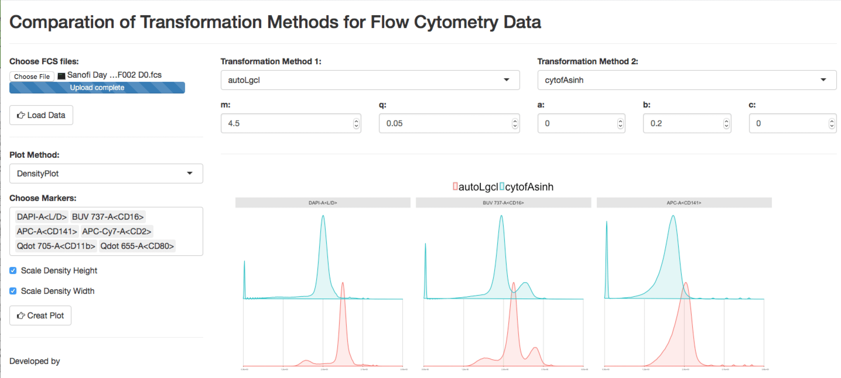
To compare the transformation methods (autoLgcl, logicle, cytofAsinh, arcsinh) for a given FCS file, a shiny APP is build and provided with link https://chenhao.shinyapps.io/TransformationComparation_shinyAPP/. A screenshot of the app is as below:

Reference

[1] From wikipedia Flow cytometry

[2] Finak G, Perez J, Weng A, Gottardo R. Optimizing transformations for automated, high throughput analysis of flow cytometry data. BMC Bioinformatics. 2010;11: 546. doi:10.1186/1471-2105-11-546.

[3] Berg RA Van Den, Hoefsloot HCJ, Westerhuis J a, Smilde AK, Werf MJ Van Der, van den Berg R a, et al. Centering, scaling, and transformations: improving the biological information content of metabolomics data. BMC Genomics. 2006;7: 142. doi:10.1186/1471-2164-7-142.

[4] Parks DR, Roederer M, Moore WA. A new “logicle” display method avoids deceptive effects of logarithmic scaling for low signals and compensated data. Cytom Part A. 2006;69: 541–551.

Session Information

sessionInfo()

## R version 3.3.2 (2016-10-31)
## Platform: x86_64-apple-darwin13.4.0 (64-bit)
## Running under: macOS Sierra 10.12.3
## 
## locale:
## [1] en_US.UTF-8/en_US.UTF-8/en_US.UTF-8/C/en_US.UTF-8/en_US.UTF-8
## 
## attached base packages:
## [1] stats     graphics  grDevices utils     datasets  methods   base     
## 
## other attached packages:
## [1] flowCore_1.40.3    ggplot2_2.2.1      wordcloud_2.5     
## [4] RColorBrewer_1.1-2 dplyr_0.5.0        knitr_1.15.1      
## 
## loaded via a namespace (and not attached):
##  [1] graph_1.52.0        Rcpp_0.12.9         cluster_2.0.5      
##  [4] magrittr_1.5        BiocGenerics_0.20.0 munsell_0.4.3      
##  [7] lattice_0.20-34     colorspace_1.3-2    rrcov_1.4-3        
## [10] R6_2.2.0            pcaPP_1.9-61        stringr_1.1.0      
## [13] highr_0.6           plyr_1.8.4          tools_3.3.2        
## [16] parallel_3.3.2      grid_3.3.2          Biobase_2.34.0     
## [19] gtable_0.2.0        DBI_0.5-1           corpcor_1.6.8      
## [22] matrixStats_0.51.0  digest_0.6.12       lazyeval_0.2.0     
## [25] assertthat_0.1      tibble_1.2          robustbase_0.92-7  
## [28] evaluate_0.10       slam_0.1-40         labeling_0.3       
## [31] stringi_1.1.2       DEoptimR_1.0-8      scales_0.4.1       
## [34] stats4_3.3.2        mvtnorm_1.0-5