A Simple Interest Calculation Challenge
Chen Hao posted on 02 Aug 2016Problem Description
Here is an interest calculation problem, for simplicity, I put the model in this way:
There is such an insurance product that ask you to put in S$2400 every year, then you will get an annual interest rate of 3% for the money you depositted, so ask how much you can earn when you take the money out after 21 years.
Codes Display
1. R version 1 (H)
I contributed my first draft of R codes as below:
saveEarn <- function(yearPut, yearInterest, yearTime){
  sum <- 0
  base <- 0
  i <- 0
  lumpSum <- function(x, rate) { x * (1+rate)}
  while(i <= yearTime){
    sum <- lumpSum(x = base, rate = yearInterest)
    cat(paste0("  --Year ", i, "; Sum:", round(sum, 2), "\n"))
    base <- sum + yearPut
    i <- i + 1
  }
  save <- yearPut * yearTime
  earn <- sum - save
  out <- c(round(save, 2), round(sum,2), round(earn, 2))
  names(out) <- c("totalMoneyPut", "totalMoneyGet", "earn")
  return(out)
}

saveEarn(yearPut=200*12, yearInterest=0.03, yearTime=21)
The output is:
--Year 0; Sum:0
  --Year 1; Sum:2472
  --Year 2; Sum:5018.16
  --Year 3; Sum:7640.7
  --Year 4; Sum:10341.93
  --Year 5; Sum:13124.18
  --Year 6; Sum:15989.91
  --Year 7; Sum:18941.61
  --Year 8; Sum:21981.85
  --Year 9; Sum:25113.31
  --Year 10; Sum:28338.71
  --Year 11; Sum:31660.87
  --Year 12; Sum:35082.7
  --Year 13; Sum:38607.18
  --Year 14; Sum:42237.39
  --Year 15; Sum:45976.52
  --Year 16; Sum:49827.81
  --Year 17; Sum:53794.64
  --Year 18; Sum:57880.48
  --Year 19; Sum:62088.9
  --Year 20; Sum:66423.57
  --Year 21; Sum:70888.27

totalMoneyPut totalMoneyGet          earn
     50400.00      70888.27      20488.27
After I sent these out, I got the reply from my colleague W:
“I think it can be implemented in a single loop, instead of an embedded function. I am not sure about R’s performance with loops, functions, and even recursion, but I think simplicity is generally preferred. “
2. C version (W)
With an invitation that “Talk is cheap, show me your codes”, W send us his C implementation
#include <stdio.h>
#include <stdlib.h>

int main (int argc, char** argv){
//int calcInt(long payment, long intRate,  long term){
        if (argc < 4){ return 1; }
        double payment, intRate, term, yr, total, interest, annInt;
        payment = atof(argv[1]); intRate = atof(argv[2]); term = atof(argv[3]);
        yr = 1; total = interest = annInt = 0;
        for (;yr <= term; yr++){
                total += payment;
                annInt = total* intRate;
                total += annInt;
                printf("Year: %2.0f\tSavings: %2.2f\tinterest: %.2f\n", yr, total, annInt);
                interest += annInt;
        }
        printf("Total saved: %.2f\tFinal balance: %.2f\tTotal interest earned: %.2f\n", total-interest, total, interest);
        return 0;
}
And he also pointed that:
“In general the time taken by each feature is like : recursion > function » loop » arithmetic (this applies at least to C or Perl/Python, I don’t know enough about R to make a serious statement) . So in C or low level languages, a simple loop will be more efficient and preferred over function and even recursion.”
3. Python version (B)
With claps and cheers, my colleague B sent his impressive python version:
interest = 0.03
injection = 2400
years = 21
sum(map(lambda x: injection * (1+interest) ** x, range(1,(years+1))))
And he highlighted that “The actual code is just one line. The rest is declaration.”
And he also gave his philosophy of coding, which I agree a lot:
“While recursion is perhaps not the fastest, it is really elegant in my opinion and rather cool to write. And I put code clarity first and optimization second. Clarity will help with debugging and spotting mistakes. No sense having buggy fast codes. “
(I should mension that actually the first version of C codes sent by W is a buggy one, attched above is a modified version.)
And my colleague M is also motivated to try using CUDA, but what a pity that we don’t have any Nvidia GPU cards here. Her weppon is too powerful for this tiny issue, but we are really interested to see using a sledgehammer to crack a nut, right?
4. R version 2 (H)
So inspired by the codes from B, I tried to implement it using one line R codes:
annualPut <- 200*12; annualInterest <- 0.03; saveYears <- 21
sum(sapply(seq_len(saveYears), function(i){annualPut*(1+annualInterest)**i}))
And I also gave me a second change to modify my R version 1 code (here I tidied the version 1 codes and remove the function declaration in function):
saveEarn <- function(annualPut, annualInterest, saveYears){
    base <- annualPut
    for(i in seq_len(saveYears)){
        lumpSum <- base*(1 + annualInterest)
        cat(paste0("  --Year ", i,
                   "; total put ", annualPut * i,
                   "; lump sum:", round(lumpSum, 2),
                   "; earn:", round(lumpSum-annualPut * i,2), "\n"))
        base <- lumpSum + annualPut
    }
    totalPut <- annualPut * saveYears
    totalEarn <- lumpSum - totalPut
    out <- c(round(totalPut, 2), round(lumpSum,2), round(totalEarn, 2))
    names(out) <- c("totalMoneyPut", "totalMoneyGet", "earn")
    return(out)
}

saveEarn(annualPut=200*12, annualInterest=0.03, saveYears=21)
5. Perl version (W)
The above one line python or R code looks cool, but they only output the final total money, it lost the yearly details. So W showed out his ultimate weapon: Perl.
($a,$term,$r) = (12*200, 21, 0.03);
printf("saved: %f\tinterest: %8.2f\tfinal: %.2f\n", $a*$_,$i=($t+=$a)*$r, $t+=$i) foreach (1..$term);
This is really cool and with all the details printed.
saved: 2400.000000	interest:    72.00	final: 2472.00
saved: 4800.000000	interest:   146.16	final: 5018.16
saved: 7200.000000	interest:   222.54	final: 7640.70
saved: 9600.000000	interest:   301.22	final: 10341.93
saved: 12000.000000	interest:   382.26	final: 13124.18
saved: 14400.000000	interest:   465.73	final: 15989.91
saved: 16800.000000	interest:   551.70	final: 18941.61
saved: 19200.000000	interest:   640.25	final: 21981.85
saved: 21600.000000	interest:   731.46	final: 25113.31
saved: 24000.000000	interest:   825.40	final: 28338.71
saved: 26400.000000	interest:   922.16	final: 31660.87
saved: 28800.000000	interest:  1021.83	final: 35082.70
saved: 31200.000000	interest:  1124.48	final: 38607.18
saved: 33600.000000	interest:  1230.22	final: 42237.39
saved: 36000.000000	interest:  1339.12	final: 45976.52
saved: 38400.000000	interest:  1451.30	final: 49827.81
saved: 40800.000000	interest:  1566.83	final: 53794.64
saved: 43200.000000	interest:  1685.84	final: 57880.48
saved: 45600.000000	interest:  1808.41	final: 62088.90
saved: 48000.000000	interest:  1934.67	final: 66423.57
saved: 50400.000000	interest:  2064.71	final: 70888.27
And he gives an even more short version if we only want the final amount:
$t=($t+$a)*(1+$r) foreach (1..$term);
Simple Benchmark Test
All looks good now, but which version do you like the most? Let’s do a simple benchmark:
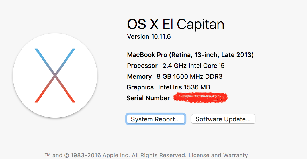
My benchmark is designed in this way, for all three variables in the model, I only change the variable years/term with value in range 100, 200, 500, 1000, 5000, 10000, 100000, 1000000, then the time elapsed for each years/term run using one of the above implementations is recorded (I only run one time for each case, only thoses looks wired I will give it a second run, this is unfair but save me time). And all the test is performed on my MacBook Pro (some information about my laptop is attached as below).

IMPORTANT NOTES: I noticed that for ALL codes except Python, the output of totoal money will be Inf when years/term goes up to 100000 or 1000000. Python actually return an error. And for some implementations like R version 2 and Python, the output is simplified (only the final amount), this can make the benchmark unfair.
1. Test Perl version
The perl codes from W is wrapped in a file testPerl.pl, contents as below:
#! usr/bin/perl

use Time::HiRes qw( time );

my $start_time = time();

my ($a,$term,$r) = @ARGV;
printf("saved: %f\tinterest: %8.2f\tfinal: %.2f\n", $a*$_,$i=($t+=$a)*$r, $t+=$i) foreach (1..$term);

my $end_time = time();
my $diff_time = $end_time - $start_time;
printf("Time elapse: %.4f\n", $diff_time);
The test example code for 100 years is perl testPerl.pl 2400 100 0.03. The time elapsed for each value of yearSpan is recorded in variable perlCost, as below:
yearSpan:   100     200     500    1000    5000   10000   1e+05   1e+06
perlCost: 0.0004  0.0022  0.0050  0.0128  0.0866  0.2450  2.0141 13.3940
NOTES: when the $term goes up to 100000, the final value becomes Inf in the print output.
2. Test C version
I saved W’s C codes in to file testC.c file, time elapsed calculation is added:
#include <stdio.h>
#include <stdlib.h>
#include <time.h>

int main (int argc, char** argv){
    //int calcInt(long payment, long intRate,  long term){
    clock_t begin = clock();
    if (argc < 4){ return 1; }
    double payment, intRate, term, yr, total, interest, annInt;
    payment = atof(argv[1]); intRate = atof(argv[2]); term = atof(argv[3]);
    yr = 1; total = interest = annInt = 0;
    for (;yr <= term; yr++){
        total += payment;
        annInt = total* intRate;
        total += annInt;
        printf("Year: %2.0f\tSavings: %2.2f\tinterest: %.2f\n", yr, total, annInt);
        interest += annInt;
    }
    printf("Total saved: %.2f\tFinal balance: %.2f\tTotal interest earned: %.2f\n", total-interest, total, interest);
    clock_t end = clock();
    double time_spent = (double)(end - begin) / CLOCKS_PER_SEC;
    printf("Time elapsed: %.4f\n", time_spent);
    return 0;
}
Then I compiled it on my mac:
gcc -o testC testC.c
The test example code for 100 years is ./cTest 2400 0.03 100. The time elapsed for each value of yearSpan is recorded in variable cCost as below:
yearSpan:  100    200    500   1000   5000  10000  1e+05  1e+06
   cCost: 0.0004 0.0007 0.0017 0.0039 0.0335 0.1075 0.8337 2.8035
NOTES: when the term goes up to 100000, the total value becomes Inf in the print output.
3. Test R version 1
Test codes for R version 1 is as below:
saveEarn <- function(annualPut, annualInterest, saveYears){
    base <- annualPut
    for(i in seq_len(saveYears)){
        lumpSum <- base*(1 + annualInterest)
        cat(paste0("  --Year ", i,
                   "; total put ", annualPut * i,
                   "; lump sum:", round(lumpSum, 2),
                   "; earn:", round(lumpSum-annualPut * i,2), "\n"))
        base <- lumpSum + annualPut
        i <- i + 1
    }
    totalPut <- annualPut * saveYears
    totalEarn <- lumpSum - totalPut
    out <- c(round(totalPut, 2), round(lumpSum,2), round(totalEarn, 2))
    names(out) <- c("totalMoneyPut", "totalMoneyGet", "earn")
    return(out)
}

yearSpan <- c(100, 200, 500, 1000, 5000, 10000, 100000, 1000000)
R1Cost <- NULL
for(years in yearSpan){
  t <- system.time(saveEarn(annualPut=200*12, annualInterest=0.03, saveYears=years))
  R1Cost <- c(R1Cost, t[3])  ## record the time elapsed
}
The time elapsed for each value of yearSpan is recorded in variable R1Cost as below:
yearSpan:  100    200    500   1000   5000  10000  1e+05  1e+06
  R1Cost: 0.002  0.005 0.013  0.027  0.171 0.332  3.702  32.343
NOTES: when the years goes up to 100000, the lumpSum value becomes Inf in the print output.
4. Test R version 2
Test code for R version 2 is as below:
yearSpan <- c(100, 200, 500, 1000, 5000, 10000, 100000, 1000000)
R2Cost <- NULL

for(years in yearSpan){
  annualPut <- 200*12; annualInterest <- 0.03; saveYears <- years
  t <- system.time({
    earn <- sum(sapply(seq_len(saveYears), function(i){annualPut*(1+annualInterest)**i}))
    cat(earn, "\n")
  })

  R2Cost <- c(R2Cost, t[3])  ## record the time elapsed
}
The time elapsed for each value of yearSpan is recorded in variable R2Cost as below:
yearSpan:  100    200    500   1000   5000  10000  1e+05  1e+06
  R2Cost: 0.0001 0.0001 0.001 0.002 0.007 0.015  0.179  2.135
NOTES: when the years goes up to 100000, the earn value becomes Inf in the print output.
5. Test Python Version
I organised B’s python codes in to one file named testPython.py with contents below:
#!/usr/bin/python
import time
import sys

start = time.time()

interest = 0.03
injection = 2400
years = int(sys.argv[1])
earn = sum(map(lambda x: injection * (1+interest) ** x, range(1,(years+1))))
print earn

end = time.time()
print end - start
Then I tested this with different years, one example is like python testPython.py 100. I run this with no problem with years less than 100000, however when I goes to python testPython.py 100000, it shows the error below:
$ python testPython.py 1000000
Traceback (most recent call last):
  File "testPython.py", line 10, in <module>
    earn = sum(map(lambda x: injection * (1+interest) ** x, range(1,(years+1))))
  File "testPython.py", line 10, in <lambda>
    earn = sum(map(lambda x: injection * (1+interest) ** x, range(1,(years+1))))
OverflowError: (34, 'Result too large')
So unlike Perl or R which give a Inf when the output value is extremely big, Python gives you an error. So I recored the time elapsed as NA for the failed cases in Python version.
The time elapsed for each value of yearSpan is recorded in variable pythonCost as below:
  yearSpan:  100    200    500   1000   5000  10000  1e+05  1e+06
pythonCost: 0.001  0.002  0.0001 0.002  0.002  0.004  NA      NA
6. Results Summary
So I organize all the time elapsed records into one R data frame as below:
testRes <- data.frame(
    yearSpan = c(100, 200, 500, 1000, 5000, 10000, 100000, 1000000),
    perlCost = c(0.0004, 0.0022, 0.005, 0.0128, 0.0866, 0.2450, 2.0141, 13.3940),
    cCost = c(0.0004, 0.0007, 0.0017, 0.0039, 0.0335, 0.1075, 0.8337, 2.8035),
    R1Cost = c(0.002, 0.005, 0.013, 0.027, 0.171, 0.332, 3.702, 32.343 ),
    R2Cost = c(0.0001, 0.0001, 0.001, 0.002, 0.007, 0.015, 0.179, 2.135),
    pythonCost = c(0.001, 0.002, 0.0001, 0.002, 0.002, 0.004, NA, NA)
)
Since pythonCost has NA values and the corresponding total money amount is Inf, I removed those NA cases and plotted the time cost using following R codes:
testRes <- data.frame(
    yearSpan = c(100, 200, 500, 1000, 5000, 10000, 100000, 1000000),
    perlCost = c(0.0004, 0.0022, 0.005, 0.0128, 0.0866, 0.2450, 2.0141, 13.3940),
    cCost = c(0.0004, 0.0007, 0.0017, 0.0039, 0.0335, 0.1075, 0.8337, 2.8035),
    R1Cost = c(0.002, 0.005, 0.013, 0.027, 0.171, 0.332, 3.702, 32.343 ),
    R2Cost = c(0.0001, 0.0001, 0.001, 0.002, 0.007, 0.015, 0.179, 2.135),
    pythonCost = c(0.001, 0.002, 0.0001, 0.002, 0.002, 0.004, NA, NA)
)

library(reshape2)
library(ggplot2)
testRes_subset <- testRes[complete.cases(testRes), ]  ## remove yearSpan = 100000, 1000000 cases
melt_testRes <- melt(testRes_subset,
                     id.vars = "yearSpan",
                     variable.name = "Language",
                     value.name = "cost")
melt_testRes$yearSpan <- factor(melt_testRes$yearSpan)
ggplot(melt_testRes, aes(x=yearSpan, y=cost, group = Language, colour=Language)) +
    geom_point() + geom_line() + theme_bw()

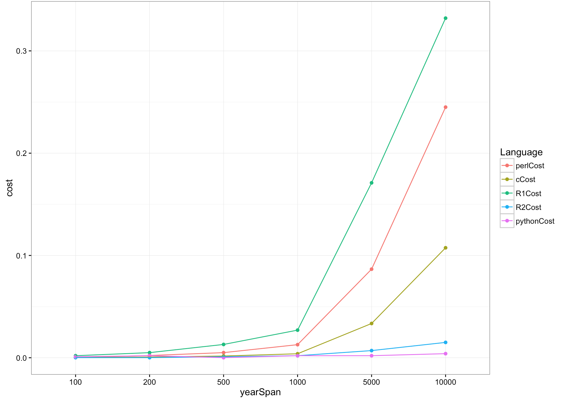
We can observe that my R1 version is the slowest, but R2 version is extremly fast (But R2 only calculate the final amount money). Which shows that a for loop in R is really expensive, using other compacted functionals like apply family will be much faster. Perl is a little bit better than R1, not so bad! Python perfoms the best, however we need to know it only print the final amount money. Surprisingly, C didn’t win in this case, but it prints a lot more details, this printings lags it behind the R2 and Python.
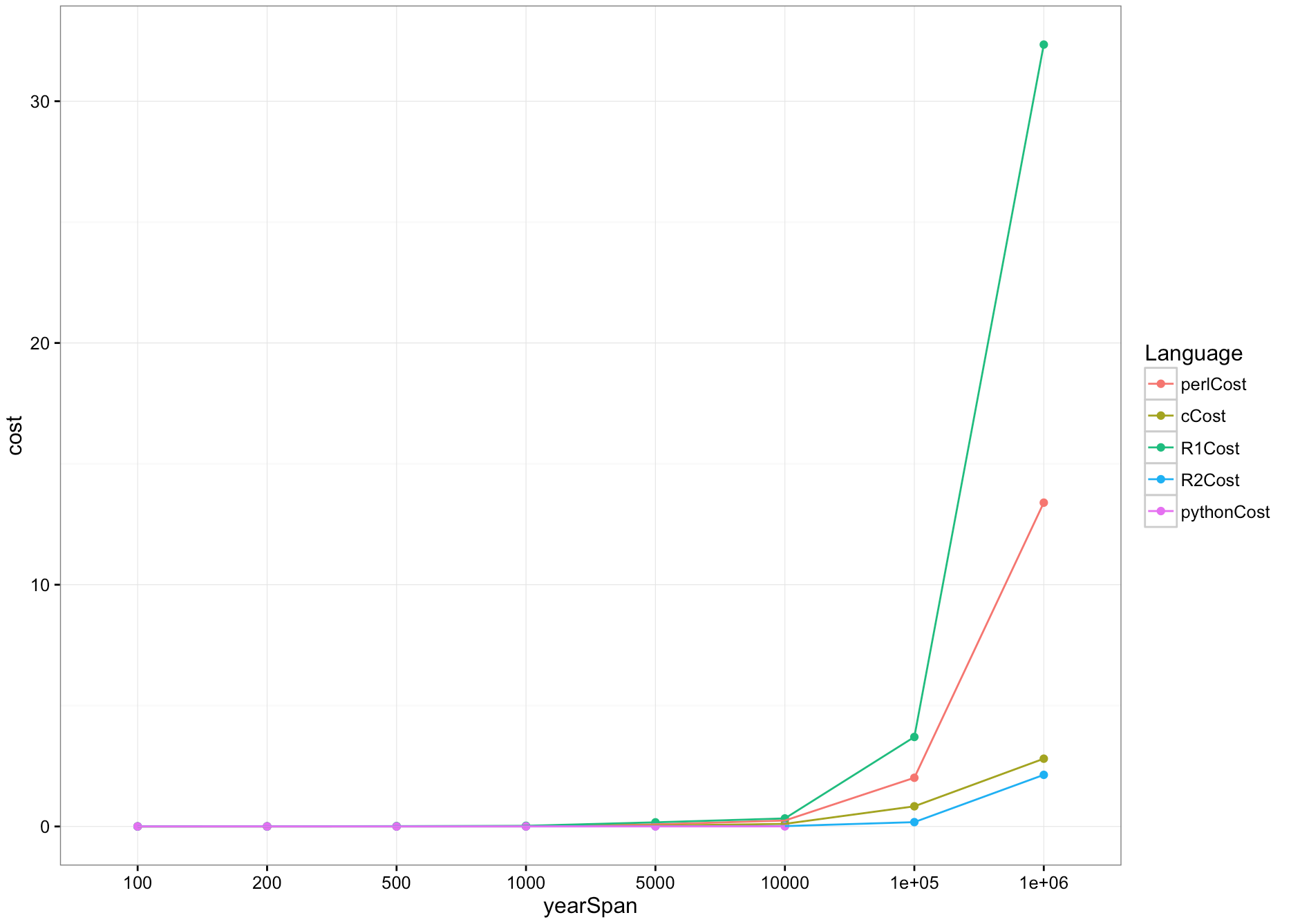
For a complete view of all tests, I also created a plot with all values:
melt_testRes <- melt(testRes,
                     id.vars = "yearSpan",
                     variable.name = "Language",
                     value.name = "cost")
melt_testRes$yearSpan <- factor(melt_testRes$yearSpan)
ggplot(melt_testRes, aes(x=yearSpan, y=cost, group = Language, colour=Language)) +
    geom_point() + geom_line() + theme_bw()

The results doesn’t change much. but once again, the output of R2 and python is not completed as other implementations, this makes them cheating in this benchmark. In a fair case, C will definitely be the winner.